tmap follows the grammar of graphics that ggplot2 is famous for. This involves the separation of data and how the data is visualized. The fundamental building block is tm_shape which takes as geospatial data argument. Other layers can then be added to it using functions like tm_borders, tm_fill etc

data("nz", package="spData") # fetch the nz, Newzealand data 
library(tmap)

tm_shape(nz) + 
  tm_fill() +             # add fill layer 
  tm_borders()            # add borders layer

The nz argument to tm_shape is the data object of type sf. You can take a peek into what it is…

str(nz)

tmap library has a function called qtm which is a handy way of quickly creating maps. For example, is the equivalent of writing tm_shape(nz) + tm_fill() + tm_borders()

It should however be noted that qtm makes controlling aesthetics much harder.

Map objects

With tmap, it is possible to store map objects in variables for later use and even adding more layers.

map_nz <- tm_shape(nz) + tm_fill() + tm_borders()
class(map_nz)

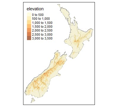
data("nz_elev", package = "spDataLarge") # fetch nz_elev from package, spDataLarge
map_nz_1 <- map_nz + tm_shape(nz_elev) + tm_raster(alpha = .7)
map_nz_1

Adding more shapes

Under international law, territorial waters extend 12 nautical miles into the sea. Let us then add map Newzealand territorial waters to its map.

library(sf) # get more functions to manipulate sf objects

nz_waters <- 
  st_union(nz) %>%  
  st_buffer(22224) %>% 
  st_cast(to = "LINESTRING") # cast to LINESTRING

map_nz_2 <- 
  map_nz_1 + tm_shape(nz_waters) + tm_lines()

map_nz_2

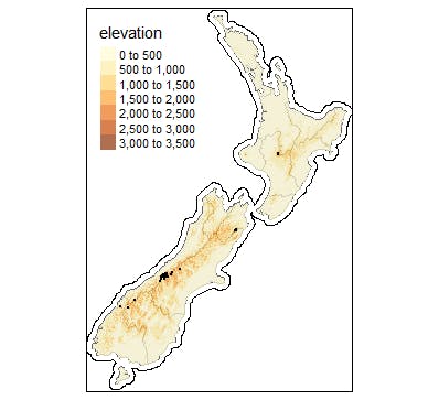
We shall now add point data on our map. This data represents hight points in Newzealand.

data("nz_height", package = "spData")

map_nz_3 <- 
  map_nz_2 + tm_shape(nz_height) + tm_dots()

map_nz_3

tmap allows you to present the maps in a grid using tmap_arrange function which takes tmap objects

tmap_arrange(map_nz_1, map_nz_2, map_nz_3)

Thanks for reading.

Reference: Geocomputation with R. (Robin Lovelace)